O_22_O Coupling between OCN and GLC components Design Document
- Tanya Reshel
- Stephen Price
- Renata McCoy
The Design Document page provides a description of the algorithms, implementation and planned testing including unit, verification, validation and performance testing. Please read Step 1.3 Performance Expectations that explains feature documentation requirements from the performance group point of view.
Design Document
In the table below, 4.Equ means Equations and Algorithms, 5.Ver means Verification, 6.Perf - Performance, 7. Val - Validation, ![]() - completed,
- completed, ![]() - in progress,
- in progress, ![]() - not done
- not done
Overview table for the owner and an approver of this feature
1.Description | Coupling between OCN and GLC components |
| 2.Owner | Jeremy Fyke (Unlicensed) |
| 3.Created | |
| 4.Equ | |
| 5.Ver | |
| 6.Perf | |
| 7.Val | |
| 8.Approver | |
| 9.Approved Date | |
| V1.0 | Accepted |
Title: O_22_O Coupling between OCN and GLC components
Requirements and Design
ACME Ocean and Ice Group
Date: 2015-9-22
Summary
Coupling of the ocean and land-ice models requires freshwater and heat fluxes to be computed at the ice-ocean interface and for the lithostatic pressure (the weight of the overlying ice) to evolve in time. In both coupled and standalone configurations, the ocean model should include the capability to simulate flows in ice-shelf cavities. This document is intended to include requirements and design for each of the three major pieces needed to compute these boundary conditions: 1) code within the ocean model to support for coupling to the land-ice model, 2) code within the land-ice model to support coupling to the ocean model and 3) code within the coupler that performs the required time averaging and regridding as well as the computation of boundary fluxes.
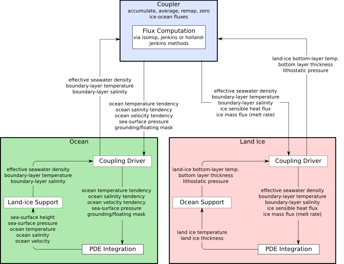
Data-flow diagram for land ice-ocean coupling (To do: update based on recent changes!)
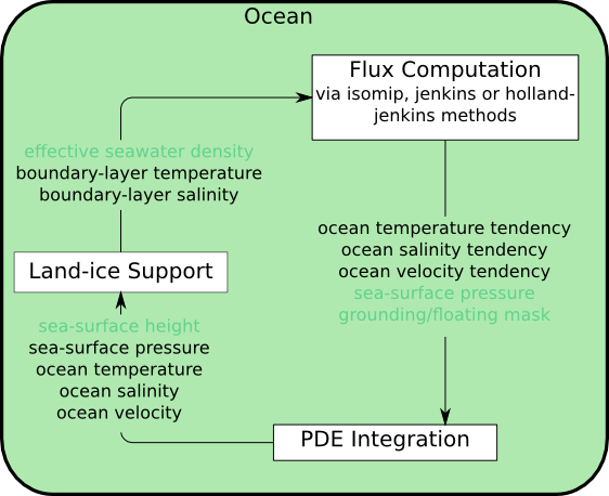
Data-flow diagram for land-ice fluxes in standalone MPAS-O.
Text in light green indicates features that are only useful with full
coupling, and are ignored in standalone MPAS-O.
2. Requirements: Support for Land-ice coupling within MPAS-O
Date last modified: 2015/09/15
Contributors: Xylar Asay-Davis, Jeremy Fyke
MPAS-O will compute the following fields on the ocean grid that need to be passed to the coupler in order to compute mass flux (melt rate) and heat fluxes at the ice-ocean interface:
- boundary-layer temperature
- boundary-layer salinity
- ocean heat-transfer velocity
- ocean salt-transfer velocity
2.1. Requirement: Jenkins et al. (2010) and Holland and Jenkins (1999) boundary conditions
Date last modified: 2015/01/30
Contributors: Xylar Asay-Davis
A run-time flag should allow the user to select between "Jenkins" or "HollandJenkins" boundary conditions. These boundary conditions are defined in Jenkins et al. (2010) and Holland and Jenkins (1999), respectively.
2.1.1 Jenkins
The Jenkins et al. (2010) boundary conditions account for conservation of salt and heat across the ice-ocean interface, which is at the pressure and salinity-dependent freezing point. The "jenkins" formulation uses constant nondimensional of heat- and salt-transfer across the sub-ice boundary layer, leading to an approximately linear dependence on velocity.
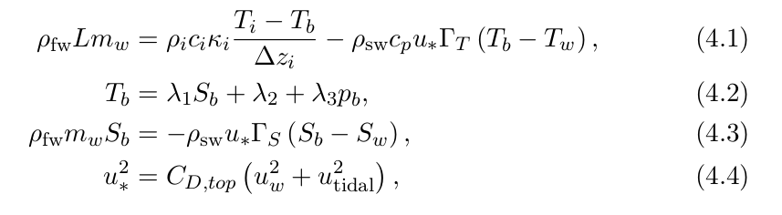
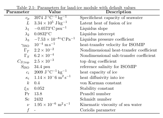
where ρfw and ρsw are the densities of freshwater and salt water, mw is the melt rate in m s-1 of water, u* is the friction velocity, uw, Tw and Sw are the velocity, temperature and salinity in the ocean grid cell adjacent to the ice-shelf interface, Tb, Sb and pb are the temperature, salinity and pressure at the ice-shelf interface. The other parameters are defined along with their default values the table above.
The freshwater flux (basal mass balance) and heat fluxes into the ocean and the ice are given by:
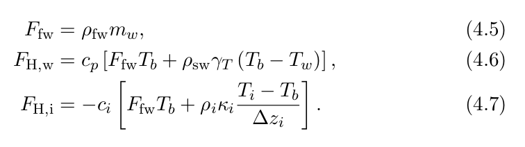
The coefficient γT = u* ΓT and γS = u* ΓS.
The solutions for Sb, Tb and mw to (4.1)-(4.3) is:
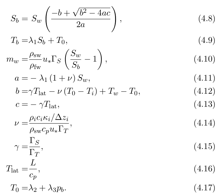
The positive root has been taken in (4.12) because salinity is always non-negative. The coefficient a is always positive (because λ1 is always negative and ν and Sw are always positive) while c is always negative, ensuring that (4.12) always produces a real, positive result.
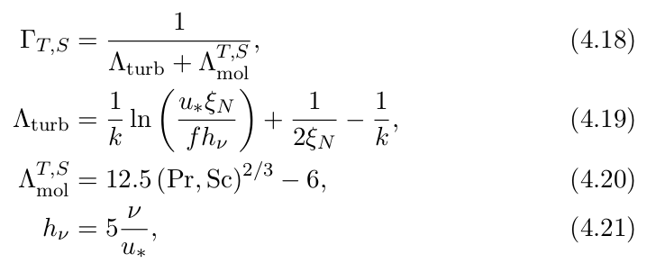
2.1.2 HollandJenkins
The Holland and Jenkins (1999) formulation includes slightly nonlinear velocity dependence in heat and salt transfer, and is commonly used in many studies including the coupled test cases of Goldberg et al. (2012a,b). The boundary conditions are as in the "jenkins" case except that ΓT and ΓS are not constants, but are given by
2.2. Requirement: Provide information for determining flotation in MPAS-LI
The sea-surface height will be allowed to evolve in MPAS-O based on the imposed pressure of the ice (see Sec. 3). This means that the ice draft (the elevation of the land ice-ocean interface) is determined by MPAS-O, rather than by MPAS-LI. In order for the location of grounding lines to be consistent between MPAS-O and MPAS-LI, MPAS-LI must use a flotation criterion that is consistent with the sea-surface height in MPAS-O and the lithostatic pressure at the ice-ocean interface.
3. Requirements: Ocean-coupling support within MPAS-LI
Date last modified: 2015/09/15
Contributors: Xylar Asay-Davis, Jeremy Fyke
MPAS-LI will compute the following fields on the land-ice grid to be passed to the coupler in order to compute mass flux (melt rate) and heat fluxes at the ice-ocean interface:
- bottom-layer temperature
- distance from bottom-layer temperature to ice-ocean interface (used to compute temperature gradient)
- ice mask
- grounded mask
- floating mask
- lithostatic pressure
The land-ice model also needs to provide the lithostatic pressure p = ρi g H as a function of space, where H is the ice-shelf thickness and ρi is the ice density.
4. Requirements: Land ice-ocean coupling support within the coupler
Date last modified: 2015/09/15
Contributors: Xylar Asay-Davis, Jeremy Fyke
4.1 Requirement: Stable evolution of boundary-layer T and S in MPAS-O
The coupler must update the freshwater and heat fluxes into the ocean frequently enough to prevent numerical instabilities associated with under-resolving feedback between the boundary-layer T and S and the fluxes. The time scale that must be resolved is given by τ ≤ HBL/mw, where HBL is the thickness of the boundary layer and mw is the melt rate (units of velocity).
4.2 Requirement: Conserving fluxes under floating ice
The coupler must be able to provide the ice sheet with melt mass and heat fluxes that is routed only to floating cells, based on the floating mask provided by MPAS-LI. The coupler must provide fluxes to MPAS-O that have been masked by the fraction of an ocean cell that is covered by floating ice.
4.3 Requirement: Fields provided to MPAS-O by the coupler
The coupler will provide the following fields to MPAS-O on its native grid:
- freshwater flux (4.5)
- heat flux (4.6)
- interface T and S, given by (4.9) and (4.8), respectively
- land ice fraction (the fraction of an ocean cell's area covered by land ice, a remapping of the ice mask)
- sea surface pressure (remapped from lithostatic pressure)
4.4 Requirement: Fields provided to MPAS-LI by the coupler
The coupler will provide the following fields to MPAS-LI on its native grid:
- basal mass balance (4.5)
- heat flux (4.7)
- effective ocean density
5. Requirements: Land-ice fluxes in standalone MPAS-O
Date last modified: 2015/01/30
Contributors: Xylar Asay-Davis
5.1. Requirement: Land-ice fluxes available in standalone MPAS-O
There should be a way that land-ice fluxes—mass (freshwater) and heat fluxes—can be computed when MPAS-O is run in standalone, idealized mode. This is needed to support idealized simulations with static ice shelves such as ISOMIP and ISOMIP+.
5.1.1 isomip
An additional flag should allow support for the ISOMIP test case (Hunter 2006). The ISOMIP boundary conditions are the simplest, neglecting the variation in salinity between the bulk ocean and the ice-ocean interface and ignoring velocity dependence in the heat-transfer coefficient:
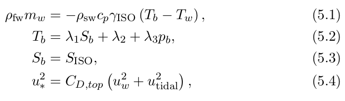
where γT = γISO is a velocity-independent constant for this configuration.
5.2. Requirement: Options for sensible heat flux into ice
Date last modified: 2015/01/31
Contributors: Xylar Asay-Davis
When MPAS-O runs in standalone mode, the user should be able to choose either of two methods for computing the sensible-heat flux into the ice: 1) the advection method of Holland and Jenkins (1999) or 2) insulating ice (with no sensible-heat flux into the ice).
5.2.1 insulating ice
The first is to set the heat diffusivity of ice, κi, to zero, meaning insulating ice and no dependence on Ti or Δzi. in (4.1), (4.7), (4.12) and (4.14).
5.2.2 Holland and Jenkins (1999) advection method for ice heat fluxes
The second approach assumes that ice is advected vertically at the melt or freezing rate and that heat diffusion within the ice is negligible. Under melting conditions, a modified version of (4.1) is applied:
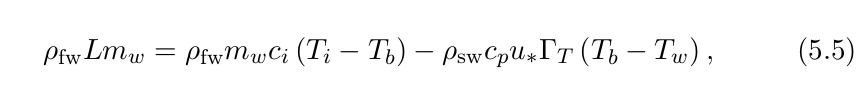
The solution to (5.5) is:
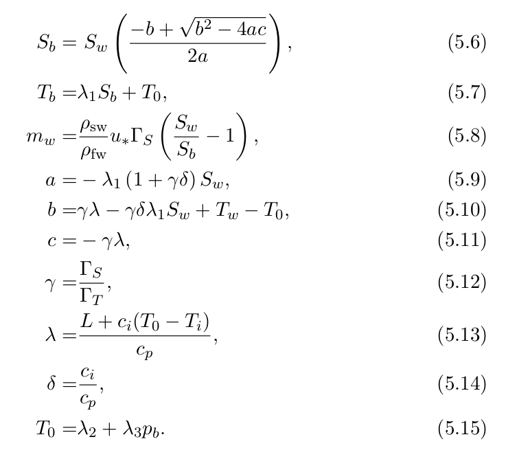
The fluxes are given by:
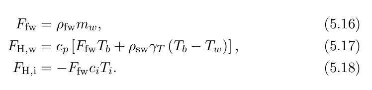
Under freezing conditions, which are determined using the sign of mw in (5.8), (4.1) is used with Ti = Tb (equivalent to insulating ice).
5.3. Requirement: Top drag
Date last modified: 2015/01/30
Contributors: Xylar Asay-Davis
MPAS-O should compute quadratic top drag under ice for inclusion in the velocity tendency.
Algorithmic Formulations
The relevant equations for the design and implementation solutions discussed below are provided in the above subsections discussing requirements.
Design and Implementation
Design solution: Coupling within MPAS-O
Date last modified: 2015/09/17
Contributors: Xylar Asay-Davis
Fields that MPAS-O passes to the coupler:
- boundary-layer temperature
- boundary-layer salinity
- ocean heat-transfer velocity
- ocean salt-transfer velocity
- effective seawater density
Fields that the coupler passes to MPAS-O:
- heat flux
- freshwater flux
- interface temperature
- interface salinity
- sea-surface pressure
- land-ice fraction
Design solution: Coupler: Stable evolution of boundary-layer T and S in MPAS-O
Date last modified: 2015/09/17
Contributors: Xylar Asay-Davis
Design solution: Coupling within MPAS-O: Jenkins et al. (2010) and Holland and Jenkins (1999) boundary conditions
Date last modified: 2015/09/17
Contributors: Xylar Asay-Davis
The boundary-layer temperature and salinity are computed as diagnostics in MPAS-O. They are computed as vertical averages of T and S over a fixed depth and (optionally) as a weighted average over nearest neighbors.
In the "jenkins" and "hollandJenkins" configurations, the ocean heat- and salt-transfer velocities (γT = u* ΓT and γS = u* ΓS) are computed as diagnostics using configuration constants and (4.18)-(4.21), respectively, to determine the nondimensional transfer coefficients ΓT and ΓS.
Design solution: Coupling within MPAS-O: determining flotation in MPAS-LI
Date last modified: 2015/09/17
Contributors: Xylar Asay-Davis
The effective seawater density (ρsw) will be computed in MPAS-O such that p = -ρsw g zss, where p is the lithosttatic pressure, supplied by MPAS-LI through the coupler, and where zss is the time-averaged sea-surface height (negative below sea-level). The effective density will be computed in regions of floating ice ("wet" regions as determined by the wetting and drying scheme and ice-covered regions as specified by the ice mask) . As part of initialization, the effective density will be extrapolated into regions of open ocean and grounded ice. The effective density will be allowed to diffuse horizontally into regions of open ocean and grounded ice through nearest-neighbor weighted averaging.
Design solution: Coupling within MPAS-LI
Date last modified: 2015/09/17
Contributors: Xylar Asay-Davis, Jeremy Fyke
The following will be time-averaged diagnostic fields computed in MPAS-LI to be passed to the coupler:
- bottom-layer temperature
- bottom-layer half-thickness
- ice mask
- grounded mask
- floating mask
- lithostatic pressure
Fields that the coupler passes to MPAS-LI:
- heat flux
- basal mass balance
- effective seawater density
- interface temperature?
(Jeremy Fyke (Unlicensed), revise as you see fit)
Design solution: Coupler: Stable evolution of boundary-layer T and S in MPAS-O
Date last modified: 2015/09/17
Contributors: Xylar Asay-Davis
The ocean model may require a faster coupling sub-interval than the land ice. The ocean coupling sub-interval τ ≤ HBL/mw of less than one day should be sufficient to prevent instability even for a rather extreme case of a 1-m boundary layer and a melt rate of 100 m/yr.
Design solution: Coupler: Conserving fluxes under floating ice
Date last modified: 2015/09/17
Contributors: Xylar Asay-Davis, Jeremy Fyke
Mass and heat fluxes will be computed on the ice-sheet grid, which is expected to be higher resolution and which has the masks for grounded and floating ice, at the ocean coupling sub-step. The fluxes will be multiplied by the floating mask before being remapped to the ocean grid. This will ensure conservation and that melt is not applied under grounded ice.
Design solution: Standalone MPAS-O: Land-ice fluxes
Date last modified: 2015/09/17
Contributors: Xylar Asay-Davis
Configuration flags allow land-ice fluxes to be computed directly in MPAS-O, rather than through the coupler. These fluxes are computed based on the same diagnostics (boundary-layer T and S, heat- and salt-transfer velocities) that would be passed to the coupler in a coupled configuration.
Three flux formulations are supported: "ISOMIP", "Jenkins" and "HollandJenkins". The ISOMIP configuration computes heat fluxes using the equations is Sec. 5.1.1. The "Jenkins" and "HollandJenkins" formulations are computed differently depending on how sensible heat into the ice is treated (see below).
Design solution: Standalone MPAS-O: Sensible heat flux into ice
Date last modified: 2015/09/17
Contributors: Xylar Asay-Davis
By default, all three flux formulations treat the ice as insulating (equivalent to κi = 0 or Ti = Tb). This is typically a good approximation, as heat fluxes into the ocean are dominated by latent heat released by melting extracted by freezing. In this configuration, The "Jenkins" and "HollandJenkins" fluxes are computed as in Secs. 2.1.1 and 2.1.2, respectively.
Optionally using a namelist flag, sensible heat fluxes into the ice can be computed using the advection method of Holland and Jenkins (1999), as described in 5.2.2. The fluxes are computed first assuming melting everywhere using (5.6)-(5.18). Then, in cells where mw < 0 (indicating freezing), the fluxes are recomputed using (4.5)-(4.17) with insulating ice.
Design solution: MPAS-O: Top drag
Date last modified: 2015/09/17
Contributors: Xylar Asay-Davis
Top drag is computed according to:
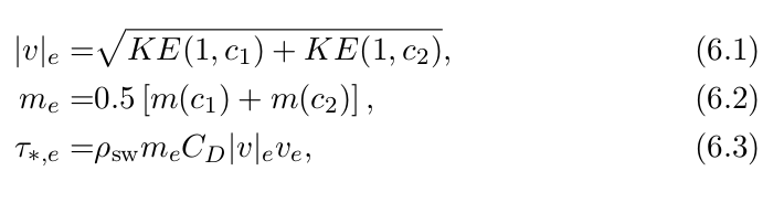
where KE(1,c) is the kinetic energy in the top level and cell c, |v|e is the velocity magnitude at edge e bordering cells c1 and c2, m(c) is the area fraction of cell c covered by land ice, me is the land-ice fraction at edge e, τ*,e is the top drag, ve is the normal velocity at edge e and CD is the drag coefficient. The top drag is added to the surface stress (which may also include wind stress). The surface stress is then distributed over multiple vertical layers based on the stress-forcing attenuation coefficient.
The top-drag magnitude is also computed as a diagnostic according to:
Planned Verification and Unit Testing
Verification and Unit Testing: Boundary Layer Physics and GLC-to-OCN Verification
Date last modified: 2015-9-22
Contributors: Xylar Asay-Davis, Mark Petersen, Stephen Price
The correct implementation of the boundary layer physics in the ocean model will be verified using the standard ISOMIP test cases.
The correct coupling between the GLC and OCN components will be verified by blah.
Planned Validation Testing
Validation Testing: Boundary Layer Physics and GLC-to-OCN Validation
Date last modified: 2015-9-22
Contributors: Xylar Asay-Davis, Mark Petersen, Stephen Price
Once suitable grids and compsets (land ice and ocean components active, data atmos., data sea ice, stub land) have been added and configured, simulations with active ocean, active ice sheet - ocean thermodynamics (but inactive land ice dynamics) will be conducted. Submarine melt rate patterns and spatially integrated submarine melt rates from these simulations will be compared to observed sub-ice shelf melt rates, as discussed in the ocean-ice diagnostics and metrics page.
Planned Performance Testing
Performance Testing: Boundary Layer Physics and GLC-to-OCN Coupling Performance
Date last modified: 2015-9-22
Contributors: Xylar Asay-Davis, Mark Petersen, Stephen Price
This introduces a new capability to the ocean model and to the climate model in general so there are no existing performance metrics. New metrics to estimate the cost of the new capability could involve:
1) calculating the cost of an existing ocean-active only simulation for which there is NO ice sheet component (e.g. the ocean stops at the ice sheet boundary)
2) calculating the cost of a similar simulation for which the ocean mesh is extended to allow for circulation beneath ice shelves and for which the boundary layer physics are active
3) comparing 1 and 2 above
References
Holland, D. M., & Jenkins, A. (1999). Modeling Thermodynamic Ice–Ocean Interactions at the Base of an Ice Shelf. Journal of Physical Oceanography, 29(8), 1787–1800. Retrieved from http://journals.ametsoc.org/doi/abs/10.1175/1520-0485(1999)029<1787:MTIOIA>2.0.CO;2
Hunter, J. (2006). Specification for test models of ice shelf cavities. Retrieved from http://staff.acecrc.org.au/~johunter/isomip/test_cavities.pdf
Jenkins, A., Hellmer, H. H., & Holland, D. M. (2001). The Role of Meltwater Advection in the Formulation of Conservative Boundary Conditions at an Ice–Ocean Interface. Journal of Physical Oceanography, 31(1), 285–296. http://doi.org/10.1175/1520-0485(2001)031<0285:TROMAI>2.0.CO;2
Jenkins, A., Nicholls, K. W., & Corr, H. F. J. (2010). Observation and parameterization of ablation at the base of Ronne Ice Shelf, Antarctica. Journal of Physical Oceanography, 40(10), 2298–2312. http://doi.org/10.1175/2010JPO4317.1