Why and how to migrate to updated atm grids and mapfiles
ACME model output (on unstructured grids) and observational data (on a variety of grids) are often remapped in a post-processing step to structured lat/lon analysis grids for use and visualization by analysis tools. There are numerous small problems with these analysis grids employed for remapping by ACME (and CESM) prior to 20150901. These flaws or limitations propagate into the weights and/or grids output by the weight-generation utility. Flawed weights produce undesirable outcomes (loss of precision, gaps) when converting from source to destination grids. All tested regridders correctly apply the weights they are supplied, and migrating to improved grids (and to mapfiles generated from those grids, e.g., by ESMF_RegridWeightGen or TempestRemap) can automatically improve both the numerical accuracy and the data and metadata completeness and consistency of the files produced by the regridding procedure. None of the problems described below affect the accuracy of the model results on the native grid. The affected grids include many CAM-FV (plain and staggered) and Gaussian grids known to be used for ACME analysis, mapfiles produced from those grids, and all mapfiles employing bilinear interpolation. The new grids improve the accuracy of diagnostics and the aesthetics of plots produced from regridded files.
Known Issues:
We identified five issues (four numerical flaws and one empty field) in the pre-migration (pre-20150901) gridfiles and mapfiles. The sixth issue is with the weight-generators themselves.
1. ACME adopted flawed CAM-FV scalar gridfiles that omitted a small strip of longitude to the east of Greenwich. This problem was identified independently by Charles Doutriaux and myself. For FV 129x256, this amounted to 0.2% of global area, that might appear as a gap or blank strip when plotted. Maps based on the flawed grids somehow reapportion area so that total area is conserved (4*pi sr), yet this necessarily redistributes weights from their true positions. This causes a mismatch between "area"- and "gw"- weighted statistics. The proper solution here is to correct the grids to avoid gaps, in this case, to restore the longitude strip to the west of Greenwich in the first zonal gridcell, and to base maps on those grids. With these grids, the gap disappears and "area"- and "gw"-weighted statistics can agree to double-precision (see examples below).
2. SCRIP introduced, and CESM and ACME inherited, coordinate storage in double precision (yay!). Unfortunately, every Gaussian grid that I have examined (T42, T62, and T85) from the CESM/CSEG grid repository has grid center latitudes (= sine of the Gaussian quadrature points) accurate to no more than eight digits. This problem also appears in files in the SCRIP distribution, and in all grid files produced by NCL that I have examined. The solution is to base latitudes on quadrature points (i.e., Legendre solutions) computed to full double precision. NCO generates SCRIP-format Gaussian grids accurate to sixteen digits, the best that double precision can reach.
3. All SCRIP and CESM-maintained Gaussian grids that I have examined (T42, T62, and T85) appear to infer gridcell interfaces as midpoints between Gaussian quadrature points/angles. Software then defines the gridcell areas from the inferred gridcell interfaces. The problem is that interfaces defined by the midpoint rule will always produce areas inconsistent with those implied by the quadrature weights. This causes a mismatch between "area"- and "gw"- weighted statistics. NCO now uses Newton-Raphson iteration (instead of the quadrature midpoints) to determine the gridcell interface location that exactly matches areas determined by the (now fully double-precision) Gaussian weights. The Newton-Raphson iteration moves interfaces by, typically, a few tenths of a degree (for moderate resolution Gaussian grids) from their previous locations as quadrature midpoints. With these grids, "area"- and "gw"-weighted statistics can be consistent and agree to double-precision (see examples below).
4. Some equi-angular lat/lon grids historically produced and used in the CESM community utilize the continuous form of the weighting function (i.e., cosine(lat)) evaluated on the discretized grid, rather than the exact discretized weight function (i.e., the difference of the sine of the latitudes bounding the zone). And some of these equi-angular lat/lon grids are used as staggered/offset grids for CAM-FV dynamics variables (e.g., U, V). All equi-angular lat/lon grids must have the same functional form for weights as the CAM-FV grid itself, since they are simply offsets of eachother. Without this correction, statistics of variables computed on the CAM-FV dynamics grid may be misdiagnosed (fxm: last sentence not yet verified). Users of all equi-angular grids, including staggered FV grids, should ensure their grids were produced with the correct weighting function. One way to do this is to verify the "area" variable, if present, exactly matches the area between the gridcell interfaces. If unsure, consider generating a new grid with the instructions below, or ask me and I will generate one for you and keep it in a standard location where others may access it.
5. For historical reasons, mapfiles generated by ESMF_RegridWeightGen (up to and including version 6.3.0rp1) using bilinear interpolation do not include complete output grid information. In particular, they lack gridcell area, because the ESMF team thought area would not be desired by users employing non-conservative mapping. However, it is helpful to include area so long as users understand that interpolative maps are non-conservative. NCO now diagnoses and adds the gridcell area to files regridded with bilinear mapfiles.
6. Weight-generators assume that great circle arcs connect grid vertices, a reasonable assumption for unstructured grids. This simplifies computing the weight of an arbitrarily shaped mesh on a sphere. However, lat/lon analysis grid vertices are connected by small circle arcs in latitude (arcs of constant latitude) and by great circles in longitude (meridians). It is difficult to map between the two systems in the general case. This limitation in state-of-the-art remapping software (ESMF_RegridWeightGen and TempestRemap) can lead to unexpected behavior (see Examples below). Unlike the five issues above, this issue has not yet been solved. Update 20170324: Recently we developed a closed-form analytic expression that can, theoretically, remap between small-circle and great-circle grids with exact conservation of area. Implementation of this formula in a remapping algorithm is on the roadmap for ncremap in 2017 (and beyond).
Why Migrate?
The new grids and mapfiles address problems 1-5, which have always existed in ACME and its predecessors (CESM, CCSM, CCM), and therefore cannot be too severe. The numerical flaws explained above can be thought of as fuzziness at the level of a few tenths of a degree in geo-referencing regridded data to the native model grid. These location errors produce only small (<< 1%) errors in regional or global statistics. So, why migrate? One aim is that diagnostics and observational evaluations with regridded data (often much more intuitive to visually evaluate than native SE grids) produce the same answers (to double precision whenever possible) as statistics computed on the native model grid. Without migration, agreement between statistics computed on the two grids (native and analysis) beyond single precision (and often worse for regional statistics) is a matter of luck and coincidence, not determinism and reproducibility. As ACME grids shift to ~1/4 degree and finer, it becomes even more important to exploit the full double precision accuracy that software can guarantee when supplied with accurate grids.
The Fix:
We generated new CAM-FV-type analysis grids with NCO (version 4.5.2 or later) and commands shown in the tables below. These grids have replaced the flawed grids on the ACME inputdata server: https://acme-svn2.ornl.gov/acme-repo/acme/mapping/grids. Gaussian grids were not originally distributed by the ACME grid/map server, though they could be found in the coupler directories. The improved Gaussian grids are now also stored on ACME's inputdata server in case they are of use to the ACME/CESM community. The improved grids are also directly available on rhea (/lustre/atlas/proj-shared/cli115/zender/grids) and yellowstone (/glade/p/work/zender/grids). UPDATE: In September 2018 we improved the Gaussian grids by ensuring the interface latitudes were exactly symmetric about the Equator. Previously the interface latitudes could have small (~10^-14) deviations from symmetry. The Gaussian latitudes (and weights) are unaffected. The newer fully symmetric grids, dated 20181001, replace the earlier Gaussian grids dated 20150901. Also, as of NCO version 4.7.7, the commands used to generate grids have changed to a simpler form invoked through ncremap rather than the hairy-old ncks invocation (which still works though). The grid generation commands below use the newer formulation for all grids, even though the FV grids have not changed at all (and are still dated 20150901).
| Old (flawed) Gridfile | New (corrected) | CAM-FV Grid Generation: |
|---|---|---|
| 129x256_SCRIP.20150901.nc | ncremap -G ttl='CAM-FV scalar grid 129x256'#latlon=129,256#lat_typ=cap#lon_typ=grn_ctr -g 129x256_SCRIP.20150901.nc | |
| 257x512_SCRIP.130510.nc | 257x512_SCRIP.20150901.nc | ncremap -G ttl='CAM-FV scalar grid 257x512'#latlon=257,512#lat_typ=cap#lon_typ=grn_ctr -g 257x512_SCRIP.20150901.nc |
ncremap -G ttl='CAM-FV scalar grid 801x1600'#latlon=801,1600#lat_typ=cap#lon_typ=grn_ctr -g 801x1600_SCRIP.20150901.nc |
| Old (flawed) Gridfile | New (corrected) | Gaussian Grid Generation: |
|---|---|---|
| T42_001005.nc | t42_scrip.20181001.nc | ncremap -G ttl='T42 Gaussian grid'#latlon=64,128#lat_typ=gss#lon_typ=grn_ctr -g t42_scrip.20181001.nc |
| T62_040121.nc | t62_scrip.20181001.nc | ncremap -G ttl='T62 Gaussian grid'#latlon=94,192#lat_typ=gss#lon_typ=grn_ctr -g t62_scrip.20181001.nc |
| T85_011127.nc | ncremap -G ttl='T85 Gaussian grid'#latlon=128,256#lat_typ=gss#lon_typ=grn_ctr -g t85_scrip.20181001.nc |
Note that ACME gridfiles and mapfiles are date-stamped. The new grid and mapfiles were produced on or after 20150724. Cubed-sphere gridfiles produced before 20150724 are still considered good. Many other atmosphere gridfiles produced before 20150724 contain the flaws mentioned above. Gridfile flaws propagate to mapfiles so in most cases mapfiles must be updated too
As of version 4.5.2, the netCDF Operator ncks generates SCRIP-format gridfiles for select grid types, including uniform/equi-angular, cap/FV, and Gaussian rectangular latitude/longitude grids. Full documentation is at http://nco.sf.net/nco.html#grid. For convenience, we summarize that functionality here. Options pertinent to the grid geometry and metadata are passed to NCO via key-value pairs prefixed by "--rgr". Pass at least six key-value pair arguments to create a fully explicitly specified, well-annotated grid. The six arguments, and their corresponding keys in parentheses, are: grid title (grd_ttl), filename to write the grid to (grid), number of latitudes (lat_nbr), number of longitudes (lon_nbr), latitude grid type (lat_typ), and longitude grid type (lon_typ). Four other arguments (the NSEW bounding box) are necessary to construct regular regional (non-global) grids, but for now we focus on global grids.
The lat_typ options for global grids are "uni" for Uniform-angle (currently same as "eqa" for Equi-angular in latitude), "cap" for Cap (same as "fv" for Finite Volume scalar grid in the CAM implementation of Lin-Rood), and "gss" for Gaussian. A Uniform (or equi-angular) in-latitude grid has constant spacing in latitude, and may have any number of latitudes. Uniform-latitude grids do not have points centered on the poles. Symmetry requires that a Uniform grids with odd numbers of latitudes center the middle latitude on the equator, while even numbers of latitudes use the Equator as an interface. A Cap grid is nearly identical to a Uniform-latitude grid, with some important data and metadata differences at the poles. Cap grids (aka CAM-FV scalar grids) are rectangular representations of Uniform-latitude grids that have a "cap" point at each pole. In order to add-up to the same latitude across the cap-point as in the rest of the zones, the polar cells in the Cap rectangular representation on disk must span half the width of the other latitudes. Moreover, that is why the center and outer interface of the polar points in the Cap grid are both labeled as 90 degrees. The contents of the polar latitude rows are often assumed to be uniform and aggregable into single "cap points" in memory. Gaussian grids must have an even number of latitudes, and therefore never have points centered on the Equator or at the poles. The lon_typ options for global grids are "grn_ctr" and "180_ctr" for the first gridcell centered at Greenwich or 180 degrees, respecitvely. And "grn_wst" and "180_wst" for Greenwich or 180 degress lying on the western edge of the first gridcell.
All grids created for this migration thus far are filename date-stamped with 20150901 to facilitate recognizing updated gridfiles and mapfiles. Full creation metadata is in the file header. Any valid netCDF file may be named as the source (e.g., in.nc). It will not be altered. The destination file (foo.nc) will be overwritten. Its contents are immaterial. Add a "-D 7" option to increase the output verbosity and check, e.g., the precision of normalization of area and latitude weights. The API for creating grids is primitive (e.g., having to repeat "--rgr") because it was quickly bolted-on to NCO. We may improve and extend the NCO API to specify other grids and maps in the future. Important updates will be noted here.
Examples:
We analyzed the global mean net TOA solar radiation for January, 1979 from an ne30 simulation on the native grid and then with old and mapfiles. Tests were performed with commands of the form "ncwa -w area -v FSNT in.nc out.nc" and "ncwa -w gw -v FSNT in.nc out.nc" where in.nc = famipc5_ne30_v0.3_00003.cam.h0.1979-01.nc for the native grid and a regridded version of that for the other mapfiles. The native grid analysis is independent of mapfile and is shown for comparison. Analysis grids produced with conservative regridding should exactly reproduce the native grid results. The "area" and "gw" rows show this is only true for a new map produced with the ESMF_RegridWeightGen (ERWG) "–user_area" switch enabled (indicated by the "_ua" in the mapfile name). The reasons for this are subtle, and are ultimately due to the approximation that the grid vertices are always joined by great circle arcs though in reality, for regular lat/lon grids, arcs of constant longitude are great circles, while arcs of constant latitude are not.
| Weighting | map_ne30np4_to_ fv129x256_aave.150418.nc | map_ne30np4_to_ fv129x256_aave.20150901.nc | map_ne30np4_to_ fv129x256_aave_ua.20150901.nc |
|---|---|---|---|
| Native | 2.441241149902344e+02 | 2.441241149902344e+02 | 2.441241149902344e+02 |
| area | 2.441241149902344e+02 | 2.441241149902344e+02 | 2.441241149902344e+02 |
| gw | 2.441210784912109e+02 | 2.441210784912109e+02 | 2.441241149902344e+02 |
| Weighting | map_ne30np4_to_ t42_aave.001005.nc | map_ne30np4_to_ t42_aave.20150901.nc | map_ne30np4_to_ t42_aave_ua.20150901.nc |
|---|---|---|---|
| Native | 2.441241149902344e+02 | 2.441241149902344e+02 | 2.441241149902344e+02 |
| area | 2.441241149902344e+02 | 2.441241149902344e+02 | 2.441241149902344e+02 |
| gw | 2.441290893554688e+02 | 2.441119842529297e+02 | 2.441241149902344e+02 |
Ignore the last column (with --user_area = "_ua" mapfiles) for now. The alert reader will see that the first two rows of both tables are identical, i.e., weighting by "area" produces identical answers whether or not one migrates to the new mapfiles. This surprised us because issues 1, 2, and 3 described above are that the old grid has a gap (for CAM-FV maps) and non-precise weights with mis-positioned centers and interfaces (for Gaussian maps). How can global-mean area-weighted answers from the flawed maps agree to double-precision with the updated maps? There are two reasons for this. First, ERWG, by default, constructs its own areas for all grids it receives. Here it somehow decides that the grids it receives are global (even though the FV grids are missing a longitude strip), and it builds its own internal representation of these grids with total surface = 4*pi sr. Second, it imposes the normalization requirement for first-order conservative remapping, meaning that it guarantees global integrals on the source and destination grids agree. In other words, it adjusts the output values of the field (FSNT, in this case) such that the integral of those values times its internally-diagnosed area-weights equals the input global integral. Some local values of FSNT in the output file are therefore scaled by an unrealistic factor, and this is non-obvious from looking at only the global integral.
The third row of both tables shows that the "gw"-weighted answers change when migrating, and that both old and new "gw"-weighted answers are incorrect, i.e., they do not agree to double-precision with the native grid. Here "gw" is the name of the variable holding the latitude-weights (which may or may not be Gaussian weights) for the output grid. Hence we prefer to call the contents of "gw" the latitude-weights. Latitude-weights are diagnosed from the user-specified gridcell interfaces of the output grid. The latitude-weighted answers change (from old to new) if the latitude-interfaces change. Latitude interfaces do not change for FV grids, and do change for Gaussian grids. All latitude-weighted answers are (still) incorrect with the new map-files (i.e., the middle column) because the latitude-weights are applied to the field-values (e.g., FSNT) consistent with the internally diagnosed area, and that area embodies the approximation that gridcell vertices are connected by great-circle arcs (whereas small-circles not great-circles connect points with the same latitude in FV and Gaussian grids). In other words, the new latitude-weights are correct but ERWG has adjusted the fields to be consistent with its internal notion of area, which is based on great-circles and is therefore incorrect for rectangular lat/lon grids.
The answers in the third column all agree to double-precision, yet we do not recommend using those mapfiles which look identical to those in the second column except that ERWG received a single additional argument, --user_areas, in producing them. This argument tells ERWG to normalize with respect to (and to output) the areas provided in the user-supplied grid-files, rather than to generate its own based on the provided grid boundares. However, ERWG can only perform remapping in a manner consistent with its internal assumption of great-circle (not small-circle) connected gridpoints so it still internally generates and uses its own area, though it outputs the user-specified area. The --user_areas switch forces ERWG to adjust the field values so that the global sum of each value, times the ratio of its user-supplied area to its internal area, is the same on input and output grids. Since the correct grid interfaces are present in the new map-files, the correct latitude-weights are diagnosed. And these weights times the fields (which now include the area-ratio factor) are correctly normalized globally (as shown) and also are correctly normalized regionally (not shown) (fxm: verify this).
Why then do we not recommend and use the mapfiles in the third column? Because they produce correct global integrals, but the have worse local precision than the middle column. Here is why: Consider a constant field, say 1.0, on the native grid. The values on the output grid must satisfy the imposed global conservation the user-supplied areas. Thus the regridding remaps 1.0 to 1.0*area_ESGF/area_True where area_ESGF is the internally diagnosed area (i.e., great-circle-based area) and area_True is the user-provided, true area (i.e., small-circle-based in latitude, great-circle-based in longitude). The ratio area_ESGF/area_True is near but not equal to 1.0. Thus the remapping turns a constant input field 1.0 into a spatially varying output value 1.0+epsilon where epsilon depends on latitude. Error characteristics of this remapping, such as the L2-norm, are inferior to those of the middle column (fxm: verify this). Moreover, a plot of the formerly constant field shows an artificial dependence on latitude which though small, is visually distracting.
To summarize, there is not yet a weight-generator which correctly handles both unstructured (great-circle-connected) grids and rectangular (small-circle-connected in latitude, great-circle in longitude) lat/lon grids. In the absence of that, the mapfiles produce weights with some drawbacks. We advocate using the map-file with the best overall error characteristics for the job at-hand. For general-purpose regridding, that is the mapfile shown in the middle-column above. If you want weights exactly valid for remapping lat/lon grids with unstructured grids (i.e., eliminating the great-circle-connected approximation), please comment below or contact Charlie Zender who will attempt to prioritize the necessary work accordingly.
Appendix: Lat/Lon Grids
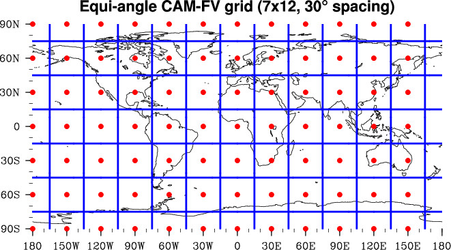
The first plot below shows the type of grid we recommended for regriding unstructured data. We chose this grid because it is the same type of grid as would be output by the CAM-FV model for all scalar fields. NCL refers to this as a "fixed" grid. It is compatible with NCL's SPHEREPACK and thus one can easily compute spherical harmonic transforms if desired.
The red dots show where the data are located, and the blue lines give the cells associated with each data point. Data may be interpreted as cell averages or as point values at the red dots. Because of the lat/lon representation, data at the poles are actually duplicated for every longitude. When viewed on the Earth, the cells containing pole points will be triangles. Good software should merge these triangles into a single n-gon containing the pole. A grid with equal spacing in both latitude and longitude will have dimensions (N+1) x 2N. Data at 180E = 180W are not duplicated in the file, and to convey this, we only plot red dots at 180W and not 180E.
You may build the SCRIP format "template" file for this grid with (in.nc can be any valid netCDF file):
ncremap -G ttl='CAM-FV scalar grid 7x12'#latlon=7,12#lat_typ=cap#lon_typ=grn_ctr -g ${DATA}/grids/${DATA}/grids/7x12_SCRIP.20150901.nc
For reference, we also show the equi-angular "offset" grid below. NCL refers to this as a "fixed offset" grid, and NCO as a Uniform grid. Many observational datasets are distributed on this grid. The CAM-FV velocities as used internally by the FV dycore are also on this grid. In CAM-FV output, "US" and "VS" will be (optionally) output on this offset grid (whose coordinates are stored as "slat" and "slon"), while "U" and "V" are interpolated to the CAM-FV scalar grid shown above.
The offset (aka Uniform) grid is somewhat easier to work with since it does not contain data at the poles. Gaussian grids look nearly identical to these offset grids, except Gaussian grids use a spacing in latitude which is not quite equi-angular. To compute spherical harmonic transforms on this grid, one must first interpolate to an equi-angle grid with points at the poles (i.e., the Cap grid above) or to a Gaussian grid. A grid with the same equal spacing in both latitude and longitude will have dimensions N x 2N.
You may build the SCRIP format "template" file for this grid with:
ncremap -G ttl='Uniform/equi-angular grid = CAM-FV velocity grid 6x12'#latlon=6,12#lat_typ=uni#lon_typ=grn_wst -g ${DATA}/grids/${DATA}/grids/6x12_SCRIP.20150901.nc 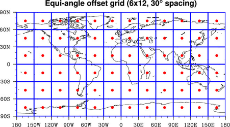
Note how the offset grid above has Greenwich on the west edge of the first gridcell. To produce the same grid except with longitude centered on Greenwich, use:
ncremap -G ttl='Uniform/equi-angular grid'#latlon=6,12#lat_typ=uni#lon_typ=grn_ctr -g ${DATA}/grids/${DATA}/grids/6x12_SCRIP.20150901.ncSuch a grid is offset from the CAM-FV scalar grid in latitude but not in longitude so it is not a CAM-FV velocity grid.