Generate the Grid Mesh (Exodus) File for a new Regionally-Refined Grid

Note: This page is PRELIMINARY. Steps described here may not work and/or there may soon be better ways to do these things.

These instructions were originally written by Mark Taylor and Colin Zarzycki and posted at https://docs.google.com/document/d/1ymlTgKz2SIvveRS72roKvNHN6a79B4TLOGrypPjRvg0/edit?usp=sharing . The basic idea is to create a .png file of the grid you want, then to use Paul Ullrich's SQuadGen code to turn it into the needed file type. For an overview of SQuadGen, see https://climate.ucdavis.edu/squadgen.php.

Basic Steps

1. Check out and compile SQuadGen from github. SQuadGen needs a version of netcdf with C++ support.    
2. Run SQuadGen (or CUBIT) to make an Exodus format “grid file”.  Here we’ll refer to that file as: newmesh.g. SQuadGen requires the user to specify the refinement area via a PNG image. 
3. To test the new grid, run an idealized problem in standalone HOMME. This requires checking out HOMME and running CMAKE regression tests to ensure it builds and runs on your platform. Details on building standalone HOMME can be found on Running E3SM on New Atmosphere Grids section 2 of generating "dual grid" template files with the fortran method.
   

How to create the .png file

1. Preferred method:
1. Here we follow a procedure developed by Oksana Guba  where we draw the PNG image on top of a background image of a cubed-sphere grid.  This allows one to have better control over the refined region’s boundaries and avoid notches and other types of glitches in the transition region.  SQuadGen generates the refinement region by using pointwise sampling of an input PNG image.  The input PNG is a grayscale representation of a regular latitude-longitude grid (under equirectangular projection) with the shading determining the level of refinement: white for the coarse grid and black where maximum refinement is desired.  Shades of gray can be used to impose an intermediate level of refinement.  To determine the refinement region on the cubed-sphere mesh, each volume on the cubed-sphere grid is sampled from the PNG image to determine the desired level of refinement on that grid.  The transition region is then built around each refinement region using "paving" tiles, with optional smoothing of edges.
   
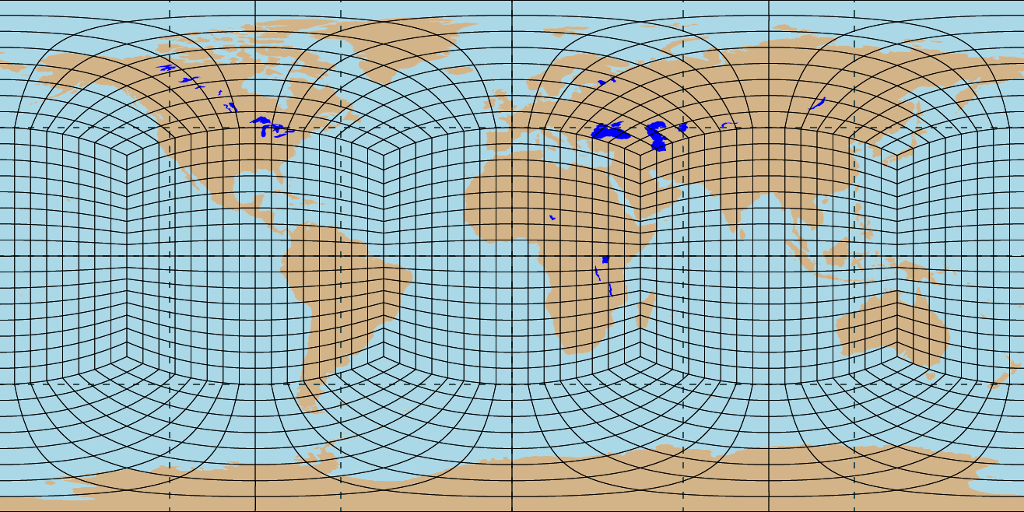
   • The following PNG image (with base grid ne16) can be used as a template for drawing your refinement region so that grid lines are parallel to cubed-sphere arcs. This PNG file will be used as a background image in Photoshop or GIMP.  The PNG of the refined region is then drawn on top of this image (in a separate layer).  You can set the transparency between layers at, i.e. 50% with the grayscale image in front of the template.  When you are ready to save the image, you can change the transparency to 0% and export the image as a PNG.
     
   •  
     
   • If desired a different "base grid" image can be generated if you want more detail as part of your template.  This can be done with "./SQuadGen --resolution <ne> --output base_grid.g", where <ne> is your desired base grid resolution.  The grid can then be plotted with the "gridplot.ncl" script and screenshotted.
   • An example PNG file with refinement over the central Atlantic is depicted below.  We will assume this file is called "newmesh.png": 
2. Use SQuadGen to create the refined grid.  The "resolution" defines the number of elements along each edge of the cubed sphere on the base grid (i.e. the coarsest resolution).  The "refine_level" defines the number of refinement levels between the coarsest resolution and the finest resolution.  Hence the resolution of the finest region is equal to <resolution>*2^-<refine_level>.
   ./SQuadGen --refine_file  newmesh.png --invert --refine_level 3 --refine_type LOWCONN \
   --resolution 16 --smooth_type SPRING --smooth_dist 3 --smooth_iter 20 \
   --output newmesh.g
3. Plot the final grid and make sure it does not have any highly deformed elements.
   • Please note:  If you use the LOWCONN option for --refine_type, try to avoid six elements around one point by editing the white parts of the PNG.  Six elements around a point is unavoidable with the CUBIT option.  
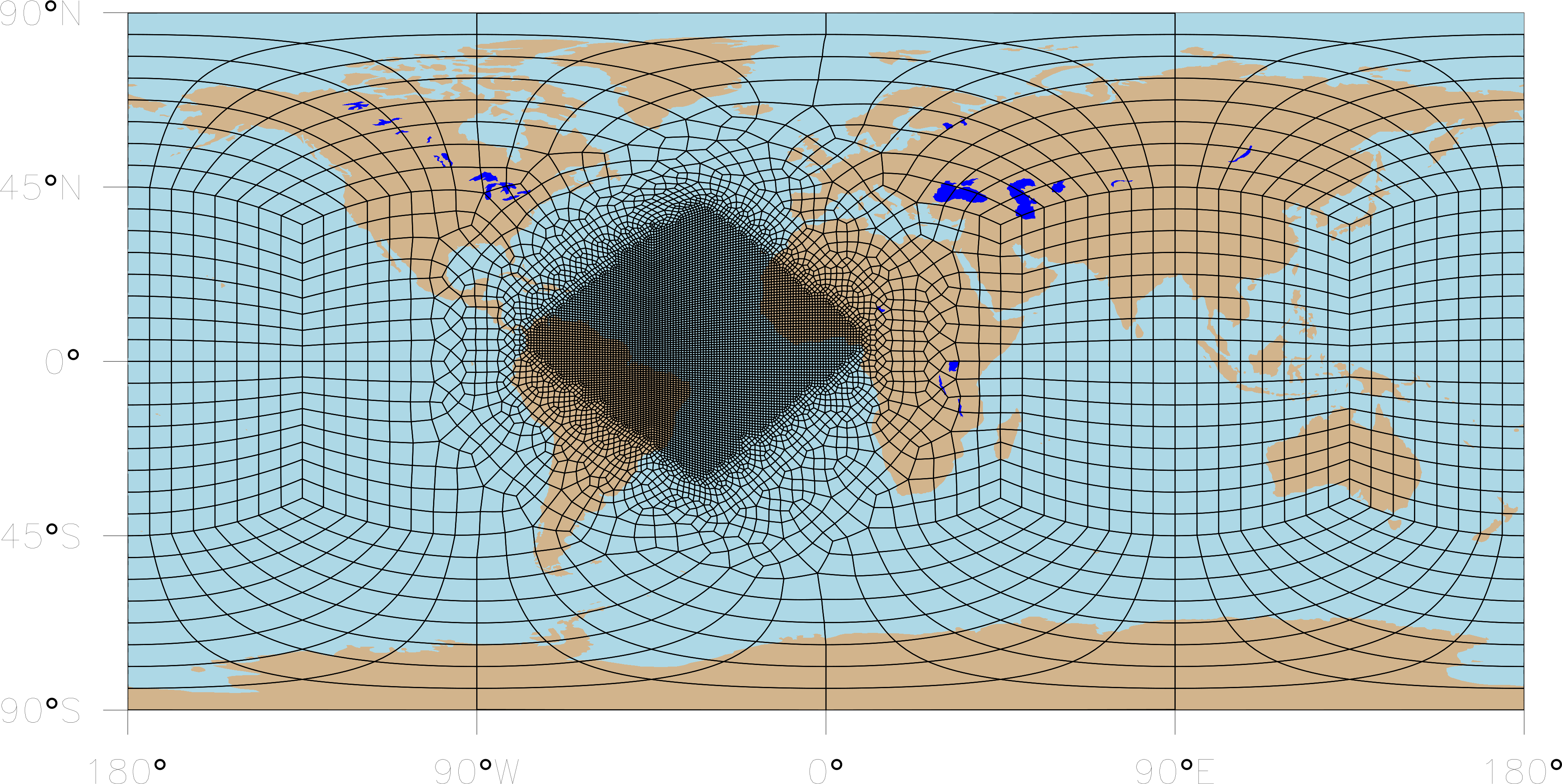
   • The mesh generated by the PNG file above is:
4. 
   

1. Alternative Method:
• An additional method may be easier if you are interested in relatively structured shapes.
• Create a white PNG with 2x1 dimensions (e.g., 2048x4096) in Paint/Paintbrush/your favorite tool. Add the refinement patch (ex: a rectangle) as a solid black shape.
• NOTE: geographical placement can be roughly controlled by running ImageMagick’s composite routine which overlays a world_map PNG (included in SQuadGen) with your refinement. Adjust newmesh.png accordingly
  composite -watermark 50% -gravity center world_map_2.png newmesh.png overlay.png
• ./SQuadGen --refine_file  newmesh.png --refine_level 3 --refine_type CUBIT \
  --resolution 15 --smooth_type SPRING --smooth_dist 3 --smooth_iter 20 \
  --output newmesh.g --invert
• NOTE: “--invert” will invert the refinement/non-refined patterns (“--invert” required for black refinement patches on white background, not needed for white on black)
• Use vi (or other text editor) to modify refine_map.dat in the SQuadGen directory. This is a map which controls the cubed-sphere elements at the level of refinement at each location. (0 indicates no refinement, 1 indicates 1 level of refinement, etc.). Here you can fix notches/cutouts in the transition region caused by the the remapping from the lat-lon projection of the PNG to the cubed sphere grid.
• ./SQuadGen --refine_file  newmesh.png --refine_level 3 --refine_type CUBIT \
  --resolution 15 --smooth_type SPRING --smooth_dist 3 --smooth_iter 20 \
  --output newmesh.g --invert --loadcsrefinementmap
  The “--loadcsrefinementmap” while force SQuadGen to use the now-modified refine_map.dat file.

Instructions for Testing a New Grid Using the Jablonowski & Williamson baroclinic instability problem.  

• Edit or modify homme/test/jw_baroclinic/run.job for your system
• This script will configure, build and run the baroclinic problem for a variety of uniform resolutions.
• Use this script to generate a working namelist.  Edit the namelist for newmesh.g:   
• ne=0
• mesh_file = “/user/path/to/newmesh.g”
• Use tensor hyperviscosity.  Enabled with a non-zero value of hypervis_scaling.  Settings are grid independent.  
• nu = 8.0e-8,  nu_div = 8.0e-8, nu_p = 8.0e-8
• hypervis_scaling=3.2
• tstep_type=5, qsplit=1, rsplit=3, hypervis_subcycle=4
• u_perturb = 1, this turns on the perturbation to generate the baroclini instability.
• Change the value of  ‘tstep’ to a value known to work with the finest resolution in newmesh.g
  • Decrease tstep until run is stable
• HOMME will interpolate the results  (u,v,T, vorticity and divergence, and tracers) and output on a NETCDF lat/lon grid and can be examined with NCL or ncview

Mesh Quality  

• After reading in an RRM mesh, HOMME running in E3SM or standalone will compute various statistics including a measure of the mesh quality/distortion, output as “Max Dinv-based element distortion”.   The equal-angle cubed-sphere grid has a value of 1.7. A high quality regionally refined grid will have a value less than 4. Getting a value less than 4 should be possible with a carefully defined refinement region and the SQuadGen ‘lowcon’ refinement option.  

Example

A jupyter notebook demonstrating creation of a new mesh is available here: https://github.com/brhillman/e3sm_grids/blob/master/notebooks/create_mesh.ipynb