See also CAM-FV Grid Overview and ATM Grid Resolution Summary
CAM-SE works with data stored at Gauss-Lobatto-Legendre (GLL) nodes. These nodes can be interpreted in several ways shown in the three various grids below. In all three gridsthe "SE native grid", "SE subcell grid" and "SE dual grid", the GLL nodes are the same (the green dots in the figure). Internally, the dycore uses the CAM-SE native grid connectivity, but the rest of CAM and ACME E3SM has no knowledge of the grid connectivity and only sees data at GLL nodes and their associated area weight. The other other types of connectivity are not used within the model, but are sometimes used by pre- and post-processing tools.
E3SM v2 adds the option to run the physics on a "physgrid", also shown below. The physgrid is a conventional finite volume (FV) grid, where each physics column is located in the center of the FV cell and represents the cell averaged quantities. The physgrid gives E3SM the flexibility to run the physics at lower or higher resolution than the dynamics.
Most native grid atmosphere output for E3SM V2 will be on the pg2 physgrid. Native grid atmosphere output from E3SM V1 is on the np4 GLL grid.
CAM-SE Native
...
Grid (GLL data)
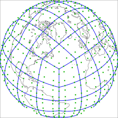
Here is a low-resolution CAM-SE grid. This is a "ne4np4" grid, meaning that it has 4x4 spectral elements in each cube face (the "ne" value), and each spectral element has a grid of 4x4 (the "np" value) Gauss-Lobatto points inside it. The blue lines show the edges of the spectral elements. CAM-SE is collocated, meaning that all variables (U,V,T, etc...) are carried around on the GLL nodes. CAM physics is computed in columns at GLL nodes. Each column has a Gauss-Lobatto weight associated with it, which can also be interpreted as an area associated with each node. The sum of these weights is 4pi (the area of the unit sphere). One can see from the figure that GLL nodes are not quite equally spaced - they cluster at the edges of the spectral elements.
Give any SE grid with N elements, the number of unique GLL nodes will be N*(np-1)^2 + 2
To map data between SE native grids and FV grids, TempestRemap should be used (see Recommended Mapping Procedures for E3SM Atmosphere Grids ). SE GLL data is not naturally represented as FV type cell averages, and thus mapping tools which only work with cell centered data (ESMF, SCRIP) should be avoided.
The PG2 "physgrid"
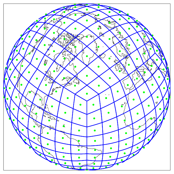
In E3SM v2, we run the physics on a finite volume grid, where each spectral element cell is further divide into subcells. PG2 computes the physics on a 2x2 FV grid within each spectral element (shown below). On the physgrid, the physics columns are located at the cell center (green dots below), but should be considered cell average values over each FV cell, rather than nodal values at the green points.
For v2 simulations, most output will be on the PG2 physgrid.
Give a SE grid with N elements, the number of unique physgrid nodes will be N*(pg)^2
The physgrid is a FV grid and can be used with any tool that works with cell centered FV data (such as ESMF map file algorithms).
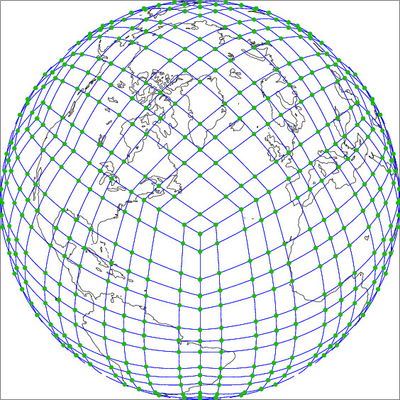
SE "subcell" grid (GLL data)
Most analysis tools and other tools can not cannot handle higher order elements such as used in CAM-SE. For these codes, we produce metadata that divide each spectral element into subcells. This subcell grid is shown below. The GLL nodes are the vertices of the subcell grid. This meta data can be used by Paraview and Visit to plot native grid CAM-SE output. The metadata is stored in a grid template file that typically has a file name of the form "<gridname>_latlon_<date>.nc" in the grids directory of the ACME E3SM inputdata server. From Euler's polyhedron formula, we know if there are N physics columns (GLL nodes), there will be N-2 subcells (all quads) and N/2-1 subcell edges.
SE "dual"
...
To remap data from the SE grid to other grids, ACME relies on ESMF mapping utilities. ESMF's conservative remapping algorithm can currently only map cell centered data. For every point in the mesh, ESMF treats that point as a cell average value, and requires that we specify its cell boundaries as a polygon. These polygons are the dual grid to the SE subcell grid. The metadata is stored in a grid template file in "SCRIP" format, that typically has a file name of the form "<gridname>_scrip-<date>.nc" in the grids directory of the ACME inputdata server.
...
grid (GLL data)
Some applications require treating the GLL nodal data as FV cell centered data. To do this, we need to construct the "dual grid" of the GLL subcell grid, resulting in a grid where each polygon contains a single GLL nodal point. This is not recommended and as one can see below is an unnatural representation of the GLL nodal data.
Constructing a SE dual grid is non-trivial and we have explored several options. :
For conservative remappingconservation, the areas of these polygons must match the weight of each GLL node. If we construct this dual grid in the usual way, by connecting the centers of all the subcells shown in the subcell grid, the areas of the cells will in general not match the GLL weights. We thus have to perform an iteration, similar to spring dynamics, tweaking the polygons until the areas are correct. We have several different algorithms to do this (examples shown below). The resulting polygons can be a little odd. First plot below (chevrons): we allow pentagons and hexagons so that the algorithm will converge faster and to more uniform cells, but this means that some of them will be slightly non-convex as some of the hexagons turn into chevrons. ESMF can handle non-convex cells, but other utilities may require they be convex. Second plot below (natural): If we only allow dual grid vertices at cell centers of the subcell grid, we get convex polygons, but they are less regular. Third plot below (pentagons): The dual grid files currently used for cubed-sphere grids in ACME E3SM selectively inserts pentagons where needed. Only the first two approaches (chevrons and natural) work with unstructured variable-resolution grids. The pentagon approach only works with cubed-sphere grids.


Meta data files: (not used directly by the
...
E3SM model, but used by the various pre- and post-processing utilities
- Exodus: <grid>.g
- NetCDF file with grid information in the Exodus format: https://github.com/gsjaardema/seacas#exodus
- This file contains a description of the spectral elements, but not the GLL or PG cells within each spectral element.
- Can be used by TempestRemap to make mapping files for GLL grids for a given np.
- Can be used by TempestRemap to make SCRIP files for PG grids.
- "latlon": <grid>_latlon_<date>.nc
- This file contains the GLL node locations and the native grid and the subcell grid connectivity
- Used by CAM's interpic_new to generate initial condition files
- Used by Paraview and Visit to plot native grid CAM-SE output
- Used by TempestRemap to create mapping files (when specifying the Jacobian to override Tempests internal reference element map)
- SCRIP: <grid>_scrip_<date.nc>
- This file contains the GLL node locations, the dual grid cell vertices and the dual grid connectivity
- Used by ESMF to create mapping files.
Tools:
- TempestRemap: https://github.com/ClimateGlobalChange/tempestremap.
- Used to make Exodus files (GLL and physgrid) and to make SCRIP files (physgrid only).
- Used to make mapping files for GLL grids directly from the Exodus file.
- Obsolete: For quasi-uniform cubed-sphere grids, ACME E3SM currently uses the "pentagons" option to construct the dual grid for making ESMF mapping files. To create these meta data grid files, we use a utility distributed with the ACME E3SM code - see acmee3sm/components/homme/test/templatestool.
- Obsolete: For RRM grids, ACME currently uses E3SM v1 used the "cheveron" option to construct the dual grid for making ESMF mapping files. To create these meta data grid files we use a Matlab program that performs a Newton interation. This matlab code is in the ACME E3SM PreAndPostProcessingScripts repo under regridding/spectral_elements_grid_utilities/
Future Plans
We note that the TempestRemap package uses an algorithm that understands both SE and FV grids (Ullrich & Taylor, MWR 2015) and can produce map files directly from the CAM-SE Native grid. It only needs the SE Native grid (the first grid shown on this page) and does not need any type of dual grid. These mapping files are more accurate since they take advantage of the SE discretization. If ACME atmosphere adopted TempestRemap mapping files, we will not need to use the SE dual grid.
Also, the "physics grid" work, when completed, will allow us to run CAM physics at cell centers of the subcell grid (instead of vertices). It will also allow us to run the physics on a subcell grid with equally spaced subcell centers. Either of these options will mean we would no longer need the SE dual grid.
...
Using TempestRemap to create Exodus and SCRIP files:
- To create the Exodus file. For cubed sphere grids with a resolution of "NE":
- GenerateCSMesh --alt --res $NE --file ne${NE}.g
- For RRM grids, the Exodus .g file is part of the model configuration and is stored along with the initial condition files in the E3SM input data server, inputdata/atm/cam/inic/homme
- To create a SCRIP file for PG2 grids from the Exodus file:
- GenerateVolumetricMesh --in ne${NE}.g --out ne${NE}pg2.g --np 2 --uniform
- ConvertMeshToSCRIP --in ne${NE}pg2.g --out ne${NE}pg2.scrip.nc
- For E3SM V2, the physics is running on the "PG2" grid. This means most output, and all coupled model mapping files need to work with PG2 grids.
- Mapping files should be created using the SCRIP file