ACME model output (on unstructured grids) and observational data (on a variety of grids) are often remapped in a post-processing step to structured lat/lon analysis grids for use and visualization by analysis tools. There are numerous small problems with these analysis grids employed for remapping by ACME (and CESM) prior to 20150901. These flaws or limitations propagate into the weights and/or grids output by the weight-generation utility. Flawed weights produce undesirable outcomes (loss of precision, gaps) when converting from source to destination grids. All tested regridders correctly apply the weights they are supplied, and migrating to improved grids (and to mapfiles generated from those grids, e.g., by ESMF_RegridWeightGen or TempestRemap) can automatically improve both the numerical accuracy and the data and metadata completeness and consistency of the files produced by the regridding procedure. None of the problems described below affect the accuracy of the model results on the native grid. The affected grids include many CAM-FV (plain and staggered) and Gaussian grids known to be used for ACME analysis, mapfiles produced from those grids, and all mapfiles employing bilinear interpolation. The new grids improve the accuracy of diagnostics and the aesthetics of plots produced from regridded files.
...
...
| Weighting | map_ne30np4_to_ t42_aave.001005.nc | map_ne30np4_to_ t42_aave.20150901.nc | map_ne30np4_to_ t42_aave_ua.20150901.nc |
|---|---|---|---|
| Native | 2.441241149902344e+02 | 2.441241149902344e+02 | 2.441241149902344e+02 |
| area | 2.441241149902344e+02 | 2.441241149902344e+02 | 2.441241149902344e+02 |
| gw | 2.441290893554688e+02 | 2.441119842529297e+02 | 2.441241149902344e+02 |
Ignore the last column (with --user_area = "_ua" mapfiles) for now. The alert reader will see that the first two rows of both tables are identical, i.e., weighting by "area" produces identical answers whether or not one migrates to the new mapfiles. This surprised us because issues 1, 2, and 3 described above are that the old grid has a gap (for CAM-FV maps) and non-precise weights with mis-positioned centers and interfaces (for Gaussian maps). How can global-mean area-weighted answers from the flawed maps agree to double-precision with the updated maps? There are two reasons for this. First, ERWG, by default, constructs its own areas for all grids it receives. Here it somehow decides that the grids it receives are global (even though the FV grids are missing a longitude strip), and it builds its own internal representation of these grids with total surface = 4*pi sr. Second, it imposes the normalization requirement for first-order conservative remapping, meaning that it guarantees global integrals on the source and destination grids agree. In other words, it adjusts the output values of the field (FSNT, in this case) such that the integral of those values times its internally-diagnosed area-weights equals the input global integral. Some local values of FSNT in the output file are therefore scaled by an unrealistic factor, and this is non-obvious from looking at only the global integral.
The third row of both tables shows that the "gw"-weighted answers change when migrating, and that both old and new "gw"-weighted answers are incorrect, i.e., they do not agree to double-precision with the native grid. Here "gw" is the name of the variable holding the latitude-weights (which may or may not be Gaussian weights) for the output grid. Hence we prefer to call the contents of "gw" the latitude-weights. Latitude-weights are diagnosed from the user-specified gridcell interfaces of the output grid. The latitude-weighted answers change (from old to new) if the latitude-interfaces change. Latitude interfaces do not change for FV grids, and do change for Gaussian grids. All latitude-weighted answers are (still) incorrect with the new map-files (i.e., the middle column) because the latitude-weights are applied to the field-values (e.g., FSNT) consistent with the internally diagnosed area, and that area embodies the approximation that gridcell vertices are connected by great-circle arcs (whereas small-circles not great-circles connect points with the same latitude in FV and Gaussian grids). In other words, the new latitude-weights are correct but ERWG has adjusted the fields to be consistent with its internal notion of area, which is based on great-circles and is therefore incorrect for rectangular lat/lon grids.
The answers in the third column all agree to double-precision, yet we do not recommend using those mapfiles which look identical to those in the second column except that ERWG received a single additional argument, --user_areas, in producing them. This argument tells ERWG to normalize with respect to (and to output) the areas provided in the user-supplied grid-files, rather than to generate its own based on the provided grid boundares. However, ERWG can only perform remapping in a manner consistent with its internal assumption of great-circle (not small-circle) connected gridpoints so it still internally generates and uses its own area, though it outputs the user-specified area. The --user_areas switch forces ERWG to adjust the field values so that the global sum of each value, times the ratio of its user-supplied area to its internal area, is the same on input and output grids. Since the correct grid interfaces are present in the new map-files, the correct latitude-weights are diagnosed. And these weights times the fields (which now include the area-ratio factor) are correctly normalized globally (as shown) and also are correctly normalized regionally (not shown) (fxm: verify this).
Why then do we not recommend and use the mapfiles in the third column? Because they produce correct global integrals, but the have worse local precision than the middle column. Here is why: Consider a constant field, say 1.0, on the native grid. The values on the output grid must satisfy the imposed global conservation the user-supplied areas. Thus the regridding remaps 1.0 to 1.0*area_ESGF/area_True where area_ESGF is the internally diagnosed area (i.e., great-circle-based area) and area_True is the user-provided, true area (i.e., small-circle-based in latitude, great-circle-based in longitude). The ratio area_ESGF/area_True is near but not equal to 1.0. Thus the remapping turns a constant input field 1.0 into a spatially varying output value 1.0+epsilon where epsilon depends on latitude. Error characteristics of this remapping, such as the L2-norm, are inferior to those of the middle column (fxm: verify this). Moreover, a plot of the formerly constant field shows an artificial dependence on latitude which though small, is visually distracting.
To summarize, there is not yet a weight-generator which correctly handles both unstructured (great-circle-connected) grids and rectangular (small-circle-connected in latitude, great-circle in longitude) lat/lon grids. In the absence of that, the mapfiles produce weights with some drawbacks. We advocate using the map-file with the best overall error characteristics for the job at-hand. For general-purpose regridding, that is the mapfile shown in the middle-column above. If you want weights exactly valid for remapping lat/lon grids with unstructured grids (i.e., eliminating the great-circle-connected approximation), please comment below or contact Charlie Zender who will attempt to prioritize the necessary work accordingly.
Appendix: Lat/Lon Grids
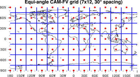
The first plot below shows the type of grid we recommended for regriding unstructured data. We chose this grid because it is the same type of grid as would be output by the CAM-FV model for all scalar fields. NCL refers to this as a "fixed" grid. It is compatible with NCL's SPHEREPACK and thus one can easily compute spherical harmonic transforms if desired.
The red dots show where the data are located, and the blue lines give the cells associated with each data point. Data may be interpreted as cell averages or as point values at the red dots. Because of the lat/lon representation, data at the poles are actually duplicated for every longitude. When viewed on the Earth, the cells containing pole points will be triangles. Good software should merge these triangles into a single n-gon containing the pole. A grid with equal spacing in both latitude and longitude will have dimensions (N+1) x 2N. Data at 180E = 180W are not duplicated in the file, and to convey this, we only plot red dots at 180W and not 180E.
You may build the SCRIP format "template" file for this grid with (in.nc can be any valid netCDF file):
ncks --rgr grd_ttl='CAM-FV scalar grid 7x12' --rgr grid=${DATA}/grids/7x12_SCRIP.20150901.nc --rgr lat_nbr=7 --rgr lon_nbr=12 --rgr lat_typ=cap --rgr lon_typ=grn_ctr ~zender/nco/data/in.nc ~/foo.nc
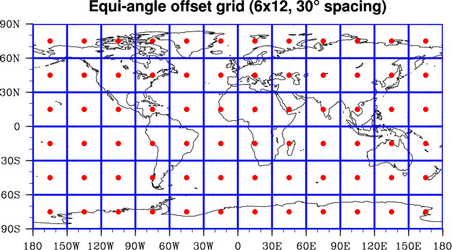
For reference, we also show the equi-angular "offset" grid below. NCL refers to this as a "fixed offset" grid, and NCO as a Uniform grid. Many observational datasets are distributed on this grid. The CAM-FV velocities as used internally by the FV dycore are also on this grid. In CAM-FV output, "US" and "VS" will be (optionally) output on this offset grid (whose coordinates are stored as "slat" and "slon"), while "U" and "V" are interpolated to the CAM-FV scalar grid shown above.
The offset (aka Uniform) grid is somewhat easier to work with since it does not contain data at the poles. Gaussian grids look nearly identical to these offset grids, except Gaussian grids use a spacing in latitude which is not quite equi-angular. To compute spherical harmonic transforms on this grid, one must first interpolate to an equi-angle grid with points at the poles (i.e., the Cap grid above) or to a Gaussian grid. A grid with the same equal spacing in both latitude and longitude will have dimensions N x 2N.
You may build the SCRIP format "template" file for this grid with:
ncks --rgr grd_ttl='Uniform/equi-angular grid = CAM-FV velocity grid 6x12' --rgr grid=${DATA}/grids/6x12_SCRIP.20150901.nc --rgr lat_nbr=6 --rgr lon_nbr=12 --rgr lat_typ=uni --rgr lon_typ=grn_wst ~zender/nco/data/in.nc ~/foo.nc
Note how the offset grid above has Greenwich on the west edge of the first gridcell. To produce the same grid except with longitude centered on Greenwich, use:
ncks --rgr grd_ttl='Uniform/equi-angular grid' --rgr grid=${DATA}/grids/6x12_SCRIP.20150901.nc --rgr lat_nbr=6 --rgr lon_nbr=12 --rgr lat_typ=uni --rgr lon_typ=grn_ctr ~zender/nco/data/in.nc ~/foo.ncSuch a grid is offset from the CAM-FV scalar grid in latitude but not in longitude so it is not a CAM-FV velocity grid.