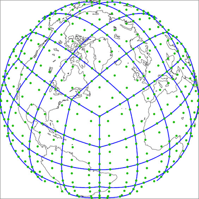
CAM-SE Native Grid
Here is a low-resolution CAM-SE grid. This is a "ne4np4" grid, meaning that it has 4x4 spectral elements in each cube face (the "ne" value), and each spectral element has a grid of 4x4 (the "np" value) Gauss-Lobatto points inside it. The blue lines show the edges of the spectral elements. The green dots show the Gauss-Lobatto points. CAM-SE is "collocated", meaning that all variables (U,V,T, etc...) are carried around on the green dots. CAM physics is computed in columns located at all the green points. Each column has a Gauss-Lobatto weight associated with it, which is also that columns area. The sum of these weights is 4pi (the area of the unit sphere). Note that the Gauss-Lobatto points are not quite equally spaced - they cluster at the edges of the spectral elements.
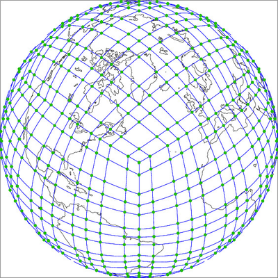
SE "subcell" grid
Most analysis tools and other tools can not handle higher order elements such as used in CAM-SE. For these codes, we produce metadata that will divide each spectral element into a subcell. This subcell grid is shown below. Note that the Gauss-Lobatto points (where CAM physics is computed) are the vertices of this grid. This meta data can be used by Paraview and Visit to plot native grid CAM-SE output. The metadata is stored in a grid template file that typically has a file name of the form "<gridname>_latlon_<date>.nc" in the grids directory of the ACME inputdata server.
SE "dual" grid
To remap data from the SE grid to other grids, ACME relies on ESMF mapping utilities. ESMF's conservative remapping algorithm can currently only map cell centered data. For every point in the mesh, ESMF treats that point as a cell average value, and requires that we specify its cell boundaries as a polygon. These polygons are the dual grid to the SE subcell grid. The metadata is stored in a grid template file in "SCRIP" format, that typically has a file name of the form "<gridname>_scrip-<date>.nc" in the grids directory of the ACME inputdata server.
For conservative remapping, the areas of these polygons must match the Gauss-Lobatto weight of each Gauss-Lobatto node. If we construct this dual grid in the usual way, by connecting the centers of all the subcells shown in the subcell grid, the areas of the cells will in general not match the Gauss-Lobatto weights. We thus have to perform an iteration, similar to spring dynamics, tweaking the polygons until the areas are correct. We have a couple of algorithms to do this, but the resulting polygons can be a little odd. The result of one of these algorithms is shown below. For this figure, we have allowed pentagons and hexagons so that the algorithm will converge faster and to more uniform cells, but this means that some of them will be slightly non-convex. ESMF can handle non-convex cells, but other utilities may require they be convex.

If we only allow triangles and quads we get convex polygons, but they are less regular:

TempestRemap
We note that the TempestRemap package uses an algorithm that understands both SE and FV grids (Ullrich & Taylor, MWR 2015) and can produce map files directly from the CAM-SE Native grid. These mapping files are more accurate since they take advantage of the SE discretization. If ACME adopts TempestRemap mapping files, we will not need to use the SE dual grid shown above.
CAM-FV Grids
We also show some plots of grids used by the Lin-Rood CAM-FV model:
The first plot below shows the grid used by CAM-FV for all scalar fields. NCL refers to this as a "fixed" gridThe red dots show where the data are located, and the blue lines give the cells associated with each data point. Data is interpreted as cell averages at the red dots. Because of the lat/lon representation, data at the poles are actually duplicated for every longitude. A grid with equal spacing in both latitude and longitude will have dimensions (N+1) x 2N. Data at 180E = 180W are not duplicated in the file, and to convey this, we only plot red dots at 180W and not 180E.

The next plot shows what NCL refers to as the fixed offset grid (aka Uniform). This is the internal CAM-FV velocity grid. CAM-FV can output these velocities if you ask for 'US' or 'VS' in the history. The 'U' and 'V' data in CAM-FV history has been interpolated to the fixed grid shown above. Gaussian grids (used by CAM-EUL) look nearly identical to these offset grids, except Gaussian grids use a spacing in latitude which is not quite equi-angular. A grid with the same equal spacing in both latitude and longitude will have dimensions N x 2N.